


今回は「CNNによる物体検出」シリーズの第一回として、最も基本的な手法であるR-CNNを解説していきます。Pythonでの実装もカバーしているので、楽しんで学んでいきましょう。
Contents
物体検出とは?
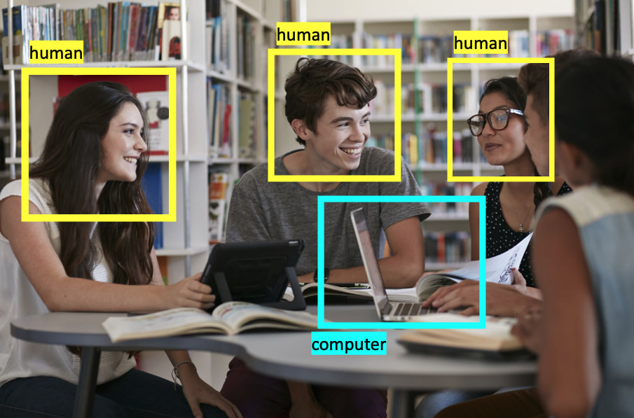
物体検出は一般物体検出とも呼ばれ、画像内の”どこ”に”何”が写っているのかを当てるタスクです。具体的には画像内の物体が存在する領域をバウンディングボックスという箱で囲い、その中に写る物体のクラスを分類します。物体検出はさまざまな分野で応用されています。自動運転における歩行者の検知や製造工場での品質管理の自動化等が実際の応用例として挙げられます。
R-CNNは2013年に発表された物体検出の手法です。この手法がこれまでのCNNを用いない手法の精度を大きく上回り、物体検出や多くのコンピュータビジョンのタスクが深層学習の時代へと突入しました。現在ではCNNだけではなく、Transformerを用いた手法まで多岐にわたる物体検出手法ですが、今回はそれらの手法の最も基本となったR-CNNを解説していきます。
R-CNNの概要
R-CNNでは物体検出を大きく3つのパートに分けて行います。まず一つ目のパートが領域提案(Region Proposal)です。そして、二つ目がCNNによる候補領域の特徴抽出部分です。最後にサポートベクターマシン(SVM)による候補内の物体の分類を行い、全体の処理が完結します。これからその一つ一つのパートを詳しく解説していきます。
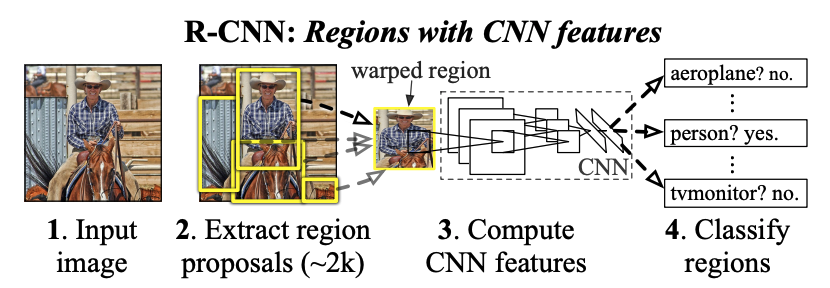
領域提案(Region Proposal)
R-CNNではSelective Searchというアルゴリズムで候補領域を抽出します。このアルゴリズムは深層学習を使用しておらず、現在では古典的なアルゴリズムといえるでしょう。今回は、このアルゴリズムの詳しい解説は省略します。PythonとOpenCVをつかって実装をしてみましたので、どのように領域提案が行われるか確認してみましょう。

※タイムアウトしてしまう場合はもう一度実行してください。
上の関数は基本的にはOpenCVが用意したSelective Searchのメソッドをそのまま使用しています。Selective Searchによって得られた候補領域の長方形を表示しています。結果のように画像内の候補領域が抽出できていることが確認できます。
CNNによる特徴抽出
Selective Searchによって抽出した候補領域の画像特徴をCNNによって取り出します。論文では比較的古典的なCNNであるAlexNetを使用しており、今回の実装でもAlexNetを使用しています。また、論文中では、あらかじめCNNをImageNetという画像認識用データセットで事前学習(pre-train)しています。PyTorchではImageNetでpre-trainされているモデルを使用することができますので、PyTorchで用意された事前学習済みAlexNetを使用することにします。
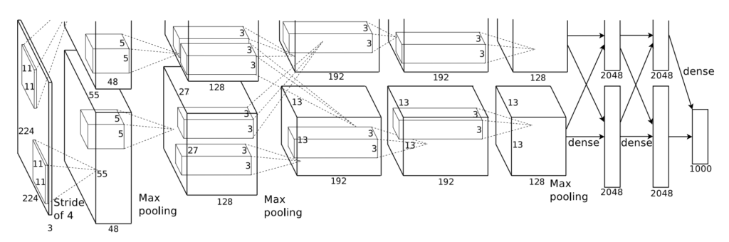
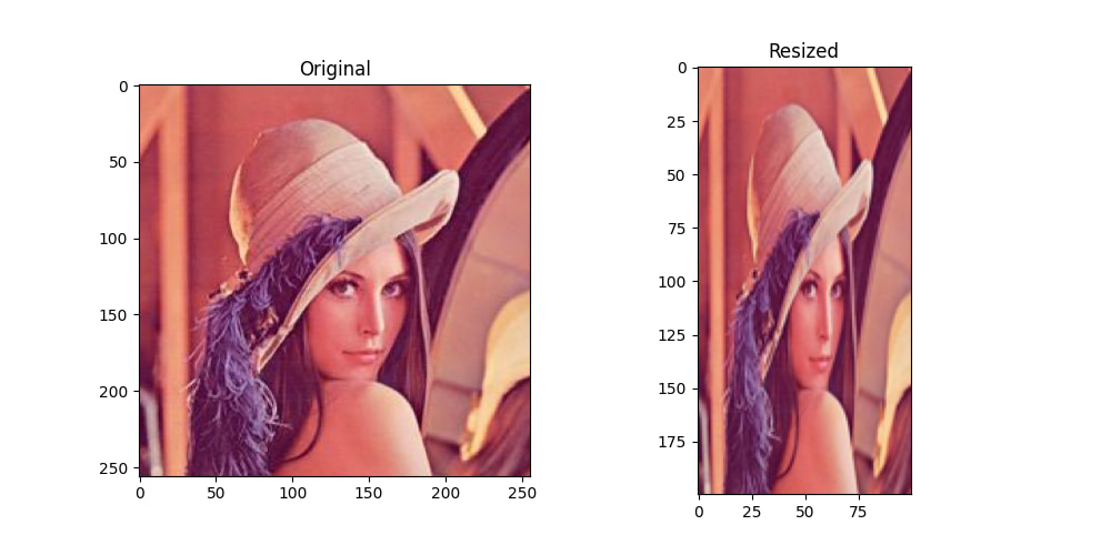
AlexNetは最後にクラス数(ImageNetであれば1000クラス)次元のベクトルを出力しますが、その出力層の前の層では4096次元のベクトルが得られます。この出力層直前の層までの特徴を次のSVMに入力するとします。つまりAlexNetからはSelective Searchから得られた候補領域に対して、それぞれ4096次元の特徴ベクトルが得られることになります。また、AlexNetは固定サイズの画像を受け取ります。これがRCNNの最大の弱点となります。 Selective Searchによって得られた候補領域はさまざまなサイズです。そして、CNNに渡される前に固定サイズにリサイズされます。ここで画像に対して不自然な変換を行わなければなりません。これが、RCNNのデメリットであり、後続の手法で改善されています。
SVMによる物体の分類
最後にCNNの特徴をもとにSVMを用いて候補領域に移っている物体のクラス分類を行います。線形SVMは分類したいクラス数+1の全結合層一層と捉えることができます。これはSVMがそれぞれのクラスに対してYes(そのクラスに該当するか?)No(そのクラスに該当しないか?)を返すためです。今回はこののSVMの部分を、PyTorchのtorch.nn.Linearモジュールを使用することで実装しました。
R-CNNの実装
データセットの作成
まずは、モデルの学習に使用するデータセットの作成を行います。今回使用するのはPASCAL VOC 2007という物体認識で広く使用されているデータセットです。PASCAL VOCは20クラスの物体に対して物体検出の学習のためのアノテーションが施されています。今回は簡単のため、今回は車のクラスのみを使用して、学習していきます。そのため、車クラスの画像のみを抽出します。以下はPASCAL VOCから車の画像とそのアノテーションデータを抽出するコードです。
import os
import shutil
import random
import numpy as np


def check_dir(data_dir):
    if not os.path.exists(data_dir):
        os.mkdir(data_dir)


suffix_xml = ".xml"
suffix_jpeg = ".jpg"

car_train_path = "./data/VOCdevkit/VOC2007/ImageSets/Main/car_train.txt"
car_val_path = "./data/VOCdevkit/VOC2007/ImageSets/Main/car_val.txt"

voc_annotation_dir = "./data/VOCdevkit/VOC2007/Annotations/"
voc_jpeg_dir = "./data/VOCdevkit/VOC2007/JPEGImages/"

car_root_dir = "./data/voc_car/"


def parse_train_val(data_path):
    """
    指定したカテゴリの画像を抽出する
    """
    samples = []

    with open(data_path, "r") as file:
        lines = file.readlines()
        for line in lines:
            res = line.strip().split(" ")
            if len(res) == 3 and int(res[2]) == 1:
                samples.append(res[0])

    return np.array(samples)


def sample_train_val(samples):
    """
    ランダムに1/10のデータを抽出
    """
    for name in ["train", "val"]:
        dataset = samples[name]
        length = len(dataset)

        random_samples = random.sample(range(length), int(length / 10))
        # print(random_samples)
        new_dataset = dataset[random_samples]
        samples[name] = new_dataset

    return samples


def save_car(car_samples, data_root_dir, data_annotation_dir, data_jpeg_dir):
    """
    目的のディレクトリに保存する
    """
    for sample_name in car_samples:
        src_annotation_path = os.path.join(voc_annotation_dir, sample_name + suffix_xml)
        dst_annotation_path = os.path.join(
            data_annotation_dir, sample_name + suffix_xml
        )
        shutil.copyfile(src_annotation_path, dst_annotation_path)

        src_jpeg_path = os.path.join(voc_jpeg_dir, sample_name + suffix_jpeg)
        dst_jpeg_path = os.path.join(data_jpeg_dir, sample_name + suffix_jpeg)
        shutil.copyfile(src_jpeg_path, dst_jpeg_path)

    csv_path = os.path.join(data_root_dir, "car.csv")
    np.savetxt(csv_path, np.array(car_samples), fmt="%s")


if __name__ == "__main__":
    samples = {
        "train": parse_train_val(car_train_path),
        "val": parse_train_val(car_val_path),
    }
    print(samples)
    # samples = sample_train_val(samples)
    # print(samples)

    check_dir(car_root_dir)
    for name in ["train", "val"]:
        data_root_dir = os.path.join(car_root_dir, name)
        data_annotation_dir = os.path.join(data_root_dir, "Annotations")
        data_jpeg_dir = os.path.join(data_root_dir, "JPEGImages")

        check_dir(data_root_dir)
        check_dir(data_annotation_dir)
        check_dir(data_jpeg_dir)
        save_car(samples[name], data_root_dir, data_annotation_dir, data_jpeg_dir)

    print("done")
次に、データセットのそれぞれの画像に対してあらかじめSelective Searchを用いて候補領域を抽出しておきます。この時に真のバウンディングボックスとの重なりが大きい候補領域はpositiveとし、重なりが小さい候補領域はnegativeとします。この重なりが大きい・重なりが小さいという指標をIoUといいます。
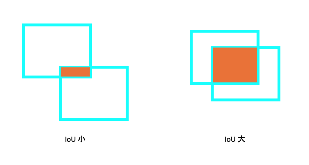
IoU(Intersection over Union)は、オブジェクト検出タスクでよく使われる評価指標です。IoUは、2つの矩形を取り、その矩形が重なる部分を「交差」、その矩形を含む大きな長方形を「并集」と呼びます。IoUは、2つの矩形の交差を、それらを含む大きな長方形の并集で割った値を表します。
IoUを計算するには、まず2つの矩形が重なる部分(交差)の面積を計算します。その後、それらを含む大きな長方形の并集の面積を計算します。最後に、交差の面積を并集の面積で割り、その結果をIoUとして計算します。IoUの計算式は以下のようになります。
IoU = 交差の面積 / 并集の面積
IoUの値は01に近いほど2つの矩形の重なりが大きく、0に近いほど重なりが小さい。つまり、IoUは2つの矩形がどの程度重なり合っているかを示しています。
以上から、データセットは以下の要素で構成されることになります。
- 画像
- 真のバウンディングボックス
- 候補領域(positiveとnegative)
次のコードは、Selective Searchによって取り出された矩形部分のIoUが閾値よりも低い場合は車ではない(negative)、IoUが大きい場合は車(positive)というようにラベルをつけていくコードです。
import numpy as np
import xmltodict
import cv2
import os
import selectivesearch


def parse_xml(xml_path):
    with open(xml_path, "rb") as f:
        xml_dict = xmltodict.parse(f)
        objects = xml_dict["annotation"]["object"]
        if isinstance(objects, list):
            bndboxes = [
                obj["bndbox"]
                for obj in objects
                if obj["name"] == "car" and int(obj["difficult"]) != 1
            ]
        elif isinstance(objects, dict):
            bndboxes = (
                [objects["bndbox"]]
                if objects["name"] == "car" and int(objects["difficult"]) != 1
                else []
            )
        return np.array(
            [
                (int(box["xmin"]), int(box["ymin"]), int(box["xmax"]), int(box["ymax"]))
                for box in bndboxes
            ]
        )


def get_selective_search(img, strategy="q"):
    gs = cv2.ximgproc.segmentation.createSelectiveSearchSegmentation()
    gs.setBaseImage(img)

    if strategy == "s":
        gs.switchToSingleStrategy()
    elif strategy == "f":
        gs.switchToSelectiveSearchFast()
    elif strategy == "q":
        gs.switchToSelectiveSearchQuality()

    rects = gs.process()
    rects[:, 2] += rects[:, 0]
    rects[:, 3] += rects[:, 1]

    return rects


def iou(pred_box, target_box):
    if len(target_box.shape) == 1:
        target_box = target_box[np.newaxis, :]

    x_a = np.maximum(pred_box[0], target_box[:, 0])
    y_a = np.maximum(pred_box[1], target_box[:, 1])
    x_b = np.minimum(pred_box[2], target_box[:, 2])
    y_b = np.minimum(pred_box[3], target_box[:, 3])

    intersection = np.maximum(0.0, x_b - x_a) * np.maximum(0.0, y_b - y_a)
    box_a_area = (pred_box[2] - pred_box[0]) * (pred_box[3] - pred_box[1])
    box_b_area = (target_box[:, 2] - target_box[:, 0]) * (
        target_box[:, 3] - target_box[:, 1]
    )

    scores = intersection / (box_a_area + box_b_area - intersection)
    return scores


def parse_annotation_jpeg(annotation_path, jpeg_path):
    # 画像を読み込み、Selective Searchを実行する
    img = cv2.imread(jpeg_path)
    rects = get_selective_search(img, "q")

    # annotationからバウンディングボックスを取得する
    bndboxs = parse_xml(annotation_path)

    # バウンディングボックスの中で最大のものを取得する
    maximum_bndbox_size = max(
        (ymax - ymin) * (xmax - xmin) for xmin, ymin, xmax, ymax in bndboxs
    )

    # iouのリストを取得する
    iou_list = [max(iou(rect, bndboxs)) for rect in rects]

    # positiveリストとnegativeリストを作成する
    positive_list = list()
    negative_list = list()
    for i, (xmin, ymin, xmax, ymax) in enumerate(rects):
        rect_size = (ymax - ymin) * (xmax - xmin)
        iou_score = iou_list[i]
        if 0 < iou_score <= 0.3 and rect_size > maximum_bndbox_size / 5.0:
            negative_list.append((xmin, ymin, xmax, ymax))
        else:
            positive_list.append((xmin, ymin, xmax, ymax))

    return positive_list, negative_list


car_root_dir = "dir/to/src data"
classifier_root_dir = "dir/to/dst data"

gs = selectivesearch.get_selective_search()
for name in ["train", "val"]:
    src_root_dir = os.path.join(car_root_dir, name)
    src_annotation_dir = os.path.join(src_root_dir, "Annotations")
    src_jpeg_dir = os.path.join(src_root_dir, "JPEGImages")

    dst_root_dir = os.path.join(classifier_root_dir, name)
    dst_annotation_dir = os.path.join(dst_root_dir, "Annotations")

    total_num_positive = 0
    total_num_negative = 0

    # 車のデータのみを記録したcsvファイル
    csv_path = os.path.join(src_root_dir, "car.csv")
    samples = np.loadtxt(csv_path, dtype="unicode")
    for sample_name in samples:

        src_annotation_path = os.path.join(src_annotation_dir, sample_name + ".xml")
        src_jpeg_path = os.path.join(src_jpeg_dir, sample_name + ".jpg")
        positive_list, negative_list = parse_annotation_jpeg(
            src_annotation_path, src_jpeg_path, gs
        )
        total_num_positive += len(positive_list)
        total_num_negative += len(negative_list)

        dst_annotation_positive_path = os.path.join(
            dst_annotation_dir, sample_name + "_1" + ".csv"
        )
        dst_annotation_negative_path = os.path.join(
            dst_annotation_dir, sample_name + "_0" + ".csv"
        )
        np.savetxt(
            dst_annotation_positive_path,
            np.array(positive_list),
            fmt="%d",
            delimiter=" ",
        )
        np.savetxt(
            dst_annotation_negative_path,
            np.array(negative_list),
            fmt="%d",
            delimiter=" ",
        )
PyTorchで使用するデータセットクラスの作成
データセットの作成が完了したら、次はPyTorchを用いてモデルを学習するのに使用するデータセットクラスを作成する必要があります。これは、学習に使用するデータセットが”画像とラベルのペア”のような単純なものではなく、候補領域の座標や、その候補領域に対するクラスラベルといった単純な物体認識のデータセットに比べ複雑な構造をしているためです。以下のコードがtorch.utils.dataのDatasetクラスをオーバーライドして作成した自作データセットクラスです。
import numpy as np
import os
import cv2
from torch.utils.data import Dataset

from utils.util import parse_car_csv


class CustomClassifierDataset(Dataset):
    def __init__(self, root_dir, transform=None):
        samples = parse_car_csv(root_dir)
        jpeg_images = []
        annotation_list = []

        for idx, sample_name in enumerate(samples):
            jpeg_image = cv2.imread(
                os.path.join(root_dir, "JPEGImages", sample_name + ".jpg")
            )

            positive_annotation_path = os.path.join(
                root_dir, "Annotations", sample_name + "_1.csv"
            )
            positive_annotations = np.loadtxt(
                positive_annotation_path, dtype=np.int, delimiter=" "
            )
            positive_annotations = (
                [positive_annotations]
                if positive_annotations.ndim == 1
                else positive_annotations
            )
            for annotation in positive_annotations:
                annotation_list.append(
                    {
                        "rect": annotation,
                        "image_id": idx,
                        "target": 1,
                    }
                )

            negative_annotation_path = os.path.join(
                root_dir, "Annotations", sample_name + "_0.csv"
            )
            negative_annotations = np.loadtxt(
                negative_annotation_path, dtype=np.int, delimiter=" "
            )
            negative_annotations = (
                [negative_annotations]
                if negative_annotations.ndim == 1
                else negative_annotations
            )
            for annotation in negative_annotations:
                annotation_list.append(
                    {
                        "rect": annotation,
                        "image_id": idx,
                        "target": 0,
                    }
                )

            jpeg_images.append(jpeg_image)

        self.transform = transform
        self.jpeg_images = jpeg_images
        self.annotation_list = annotation_list

    def __getitem__(self, index: int):
        annotation = self.annotation_list[index]
        xmin, ymin, xmax, ymax = annotation["rect"]
        image_id = annotation["image_id"]
        target = annotation["target"]
        image = self.jpeg_images[image_id][ymin:ymax, xmin:xmax]

        if self.transform:
            image = self.transform(image)

        return image, target

    def __len__(self):
        return len(self.annotation_list)
分類器(SVM)の学習
SVMの学習は基本的にニューラルネットワークにように勾配方で重みとバイアスを調整することで行います。一つ大きく異なるのは損失関数です。ニューラルネットワークによる画像分類では、一般的にクロスエントロピー損失を使用します。一方で、線形SVMではマージン(境界線からサポートベクトルまでの距離)を最大化することを考えます。ここで導入されるのがヒンジ損失です。ヒンジ損失は以下の式で表されます。これは(現在のマージンと設定した最大マージン、の最大値)+正則化項を計算しています。学習は時間がかかるため実行はできませんが、コードを参考までに記載しておきます。
ここで、は正解ラベル、
はモデルの予測値です。実際には重みの正則化項が加わります。
いよいよSVMを学習する準備が整いました。 Selective Searchによって特徴領域を取り出し、AlexNetによって矩形領域の特徴ベクトルを得ます。そして最後に線形SVMによって分類を行い、ヒンジ損失を元に学習を進めていきます。以下にコードを記載します。実行の際には先ほど作成したカスタムデータセットクラスをimportしてください。
import copy
import os
import random
import torch
import torch.nn as nn
import torch.optim as optim
from torch.utils.data import DataLoader
import torchvision.transforms as transforms
from torchvision.models import alexnet

from custum_classifier_dataset import CustomClassifierDataset


def load_data(data_root_dir):
    # データの前処理を定義する
    transform = transforms.Compose(
        [
            transforms.ToPILImage(),
            transforms.Resize((227, 227)),
            transforms.RandomHorizontalFlip(),
            transforms.ToTensor(),
            transforms.Normalize((0.5, 0.5, 0.5), (0.5, 0.5, 0.5)),
        ]
    )

    # データを格納する辞書を用意する
    data_loaders = {}
    data_sizes = {}
    remain_negative_list = list()
    # 学習データと検証データを取得する
    for name in ["train", "val"]:
        data_dir = os.path.join(data_root_dir, name)

        # データをロードする
        data_set = CustomClassifierDataset(data_dir, transform=transform)
        # 学習データの場合は、負のサンプルをランダムに選択する
        if name is "train":
            positive_list = data_set.get_positives()
            negative_list = data_set.get_negatives()

            init_negative_idxs = random.sample(
                range(len(negative_list)), len(positive_list)
            )
            init_negative_list = [
                negative_list[idx]
                for idx in range(len(negative_list))
                if idx in init_negative_idxs
            ]
            remain_negative_list = [
                negative_list[idx]
                for idx in range(len(negative_list))
                if idx not in init_negative_idxs
            ]

            data_set.set_negative_list(init_negative_list)
            data_loaders["remain"] = remain_negative_list

        # データローダーを作成する
        data_loader = DataLoader(
            data_set,
            batch_size=len(data_set),
            num_workers=8,
            drop_last=True,
        )
        data_loaders[name] = data_loader
        data_sizes[name] = len(data_set)
    return data_loaders, data_sizes


def hinge_loss(outputs, labels):
    num_labels = len(labels)
    correct_outputs = outputs[range(num_labels), labels]
    correct_outputs = correct_outputs.unsqueeze(0).T

    margin = 1.0
    margins = outputs - correct_outputs + margin
    max_margins, _ = torch.max(margins, dim=1)
    loss = torch.sum(max_margins) / len(labels)

    return loss


def train_model(
    data_loaders, model, criterion, optimizer, lr_scheduler, num_epochs=25, device=None
):
    best_acc = 0.0

    for epoch in range(num_epochs):
        for phase in ["train", "val"]:
            if phase == "train":
                model.train()
            else:
                model.eval()

            running_loss = 0.0
            running_corrects = 0

            for inputs, labels in data_loaders[phase]:
                inputs = inputs.to(device)
                labels = labels.to(device)

                optimizer.zero_grad()
                with torch.set_grad_enabled(phase == "train"):
                    outputs = model(inputs)
                    _, preds = torch.max(outputs, dim=1)
                    loss = criterion(outputs, labels)

                    if phase == "train":
                        loss.backward()
                        optimizer.step()

                running_loss += loss.item() * inputs.size(0)
                running_corrects += torch.sum(preds == labels.data)
            if phase == "train":
                lr_scheduler.step()

            epoch_loss = running_loss / data_sizes[phase]
            epoch_acc = running_corrects.double() / data_sizes[phase]
            print(f"{phase} Loss: {epoch_loss:.4f} Acc: {epoch_acc:.4f}")

            if phase == "val" and epoch_acc > best_acc:
                best_acc = epoch_acc
                best_model_weights = copy.deepcopy(model.state_dict())

        torch.save(best_model_weights, "./models/best_linear_svm_alexnet_car.pth")


device = torch.device("cuda:0" if torch.cuda.is_available() else "cpu")
data_loaders, data_sizes = load_data("./data/classifier_car")

model_path = "./models/alexnet_car.pth"
model = alexnet()
num_classes = 2
num_features = model.classifier[6].in_features
model.classifier[6] = nn.Linear(num_features, num_classes)
model.load_state_dict(torch.load(model_path))
model.eval()

for param in model.parameters():
    param.requires_grad = False

model.classifier[6] = nn.Linear(num_features, num_classes)

model = model.to(device)

hinge_loss_fn = hinge_loss

optimizer = optim.SGD(model.parameters(), lr=1e-4, momentum=0.9)
lr_scheduler = optim.lr_scheduler.StepLR(optimizer, step_size=4, gamma=0.1)

train_model(
    data_loaders=data_loaders,
    model=model,
    criterion=hinge_loss_fn,
    optimizer=optimizer,
    lr_scheduler=lr_scheduler,
    num_epochs=10,
    device=device,
)
SVMによる分類の実行例
今回、SVMの学習には時間がかかるためweb上の実行はできませんが、推論部分であれば短時間で実行可能です。次のコードはSVMによる分類部分の例です。学習済みのSVMとAlexNetを使用してSelective Searchから得られた領域をAlexNetによって特徴抽出し、SVMで分類する部分までを実行しています。

検出結果を良くするための工夫
SVMによる候補領域の分類結果を見るとバウンディングボックスが大量に発生し、お世辞にも正しく物体検出できているとは言えません。さらに検出精度を高めるために、二つの工夫を加えます。まず一つ目の工夫が「Non-Maximum Suppression」です。この処理はバウンディングボックスの重なりを解消するための処理です。具体的にはIoU(Intersection over Union)が閾値を超えた部分を一つのバウンディングボックスにします。
二つ目の工夫が、「分類器の閾値処理」です。SVMの出力スコア(入力データが各クラスに分類されるスコア)が閾値以下のバウンディングボックスを無視するように処理します。この処理によって、分類器が曖昧に分類しているバウンディングボックスを排除することができます。
また論文ではバウンディングボックスのオフセットを予測する層を追加で学習することで検出結果を高めることができると述べています。今回は簡単のため、この部分は省略することとします。
推論を行ってみる
実際にRCNNの推論部分を頭から実行してみます。簡単なサンプルであればちゃんと物体検出ができているのが確認できます。一方で、複雑に物体が配置されているサンプルでは精度が今ひとつで、推論速度も最新の手法より遅いです。次回以降紹介する発展系の手法と比較することで物体検出の手法の進化を実感していただければと思います。

さいごに
今回はCNNを使用した物体検出の手法であるRCNNの紹介と実装を行いました。次回以降ではさらに発展した手法を紹介していきますので、ぜひチェックしてみてください。
参考文献
- Rich feature hierarchies for accurate object detection and semantic segmentation. Ross Girshick, Jeff Donahue, Trevor Darrell, Jitendra Malik. CVPR 2014
- 実装はgithubリポジトリ: https://github.com/object-detection-algorithm/R-CNN を参考にしました。


